bayesAB 0.7.0
Quick announcement that my package for Bayesian AB Testing, bayesAB, has been updated to 0.7.0 on CRAN. Some improvements on the backend as well a few tweaks for a more fluid UX/API. Some links:
Now, on to the good stuff.
Why should we care about priors?
Most questions I've gotten since I released bayesAB have been along the lines of:
- Why/how is Bayesian AB testing better than Frequentist hypothesis AB testing?
- Why do I need priors?
- Do I really really really need priors?
- How do I choose priors?
Question 1 has a few objective and a few subjective answers to it. The main benefits are ones that I've already highlighted in the README/vignette of the bayesAB package. To briefly summarize, we get direct probabilities for A > B (rather than p-values) and distributions over the parameter estimates rather than point estimates. Finally, we can also leverage priors which help with the low sample size and low base rate problems.
To start, let's go back to what a prior actually is in a Bayesian context. There are countless mathematical resources out there (including part of my previous blog post) so I'll only about this conceptually. Simply put, a prior lets you specify some sort of, ahem, prior information about a certain parameter so that the end posterior on that parameter encapsualtes both the data you saw and the prior you inputted. Priors can come from a variety of places including past experiments, literature, and domain expertise into the problem. See this blogpost for a great example of somebody combining their own past data and literature to form very strong priors.
Priors can be weak or strong. The weakest prior will be completely objective and thus assign an equal probability to each value for the parameter. Examples of this include a Beta(1, 1) prior for the Bernoulli distribution. In these cases, the posterior distribution is completely reliant on the data. A strong prior will convey a very precise belief as to where a parameter's values may lie. For example:
library(bayesAB)

plotBeta(1000, 1000)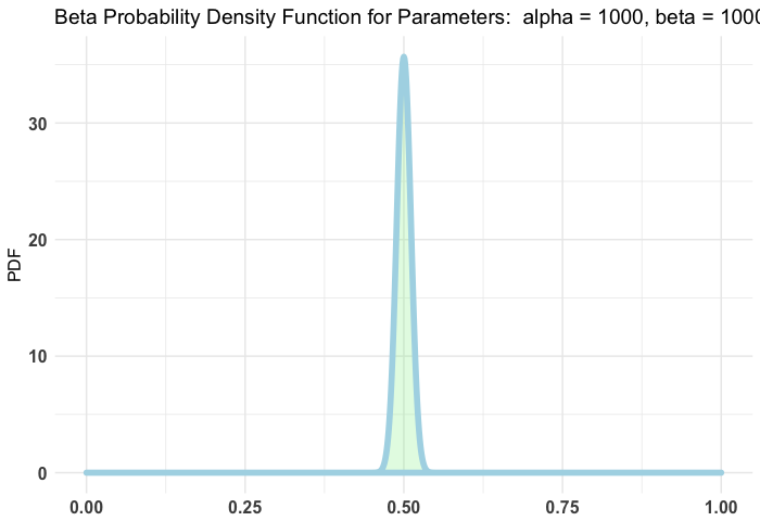
The stronger the prior the more say it has in the posterior distribution. Of course, according to the Bernstein–von Mises theorem the posterior is effectively independent of the prior once a large enough sample size has been reached for the data. How quickly this is the case depends on the strength of your prior.
Do you need (weak/strong) priors? Not necessarily. You can still leverage the interpretability benefits of Bayesian AB testing even without priors. At worst, you'll also get slightly more pertinent results since you can parametrize your metrics as the appropriate distribution random variable. However, without priors of some kind (and to be clear, not random bullshit priors either) you run into similar issues as with Frequentist AB testing, namely Type 1 and Type 2 errors. A Type 1 error is calling one version better when it really isn't, and a Type 2 error is calling a better version equal or worse. Both typically arise from low sample size/base rate and are controlled by reaching appropriate sample size as per a power calculation.
So what can we do?
Have no fear! Even without good and/or strong priors there are still ways to control for false positives and all that good stuff. We use something called Expected Posterior Loss or "based on the current winner, what is the expected loss you would see should you choose wrongly". If this value is lower than your threshold of caring (abs(A - b)) then you can go ahead and call your test. This value implictly encompasses the uncertainty about your posteriors.
Okay cool, that roughly answers Questions 1-4 in some order.
Simulation
Let's do a quick simulation to illustrate some of the above points. Let's make three examples: weak priors, strong priors, and diffuse priors (quick tip: the Jeffrey's Prior of a Gamma distribution is Gamma(eps, eps) where eps is smallllll). We'll be taking 2 x 100 samples from a Poisson distribution with the same $\lambda$ parameters. The strong and weak priors will be centered around this value of 2.3.
library(magrittr)

n <- 1e3
out_weaker_priors <- rep(NA, n)
out_stronger_priors <- rep(NA, n)
out_diffuse <- rep(NA, n)

getProb <- function(x) summary(x)$probability$Lambda

for(i in 1:n) {
  A <- rpois(100, 2.3)
  B <- rpois(100, 2.3)

  out_weaker_priors[i] <- bayesTest(A, B, priors = c('shape' = 23, 'rate' = 10), distribution = 'poisson') %>%
    getProb

  out_stronger_priors[i] <- bayesTest(A, B, priors = c('shape' = 230, 'rate' = 100), distribution = 'poisson') %>%
    getProb

  out_diffuse[i] <- bayesTest(A, B, priors = c('shape' = 0.00001, 'rate' = 0.00001), distribution = 'poisson') %>%
    getProb
}

out_weaker_priors <- ifelse(out_weaker_priors <= 0.05 | out_weaker_priors >= .95, 1, 0)
out_stronger_priors <- ifelse(out_stronger_priors <= 0.05 | out_stronger_priors >= .95, 1, 0)
out_diffuse <- ifelse(out_diffuse <= 0.05 | out_diffuse >= .95, 1, 0)
Now, A and B shouldn't have any difference between the two but occasionally we will see a Type 1 error. That's what the bottom 3 lines are doing. If P(A > B) is <=0.05 or >= .95 we call one of the recipes "significantly" better. Observe what happens with each case of prior.
mean(out_weaker_priors)## [1] 0.081mean(out_stronger_priors)## [1] 0.02mean(out_diffuse)## [1] 0.095The diffuse priors have the most Type 1 errors, followed by the weak priors, followed by the strong priors; to be expected.
Finally, we can fit another bayesTest (:D) to determine whether the differences between Type 1 error percents across priors are different from one another.
t1 <- bayesTest(out_diffuse, out_weaker_priors, priors = c('alpha' = 1, 'beta' = 1), distribution = 'bernoulli')
t2 <- bayesTest(out_diffuse, out_stronger_priors, priors = c('alpha' = 1, 'beta' = 1), distribution = 'bernoulli')

plot(t1)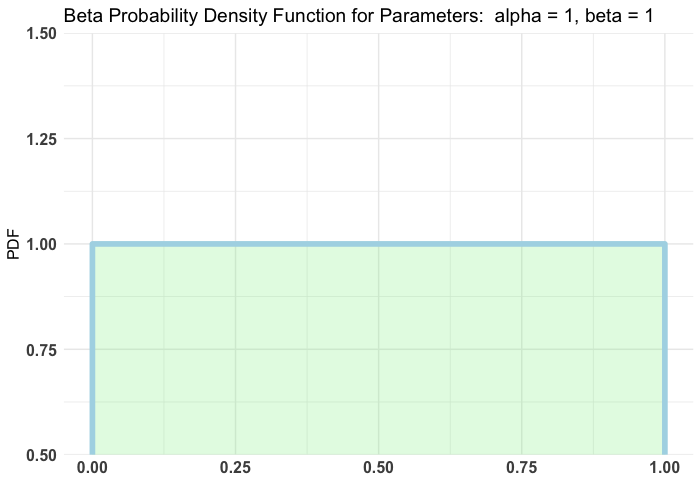
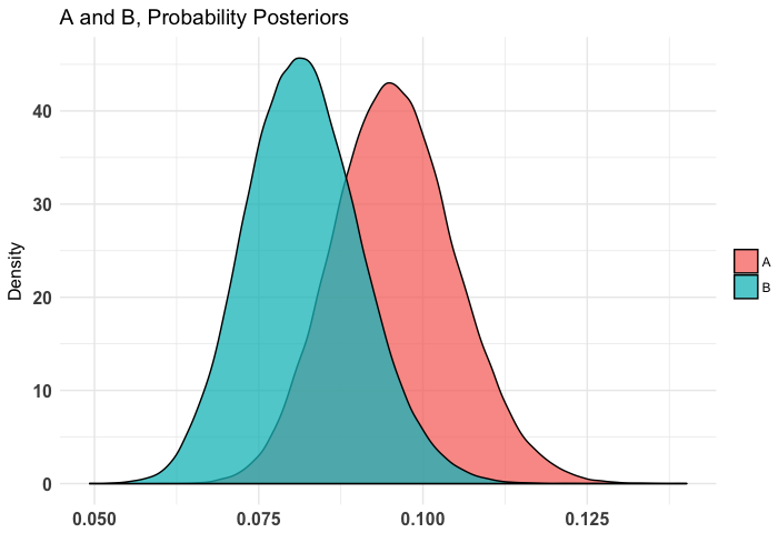
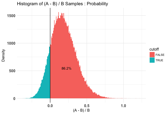
plot(t2, priors = FALSE)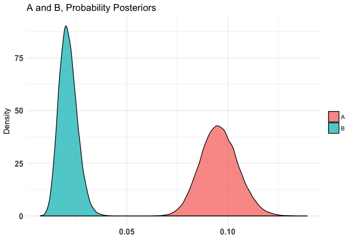
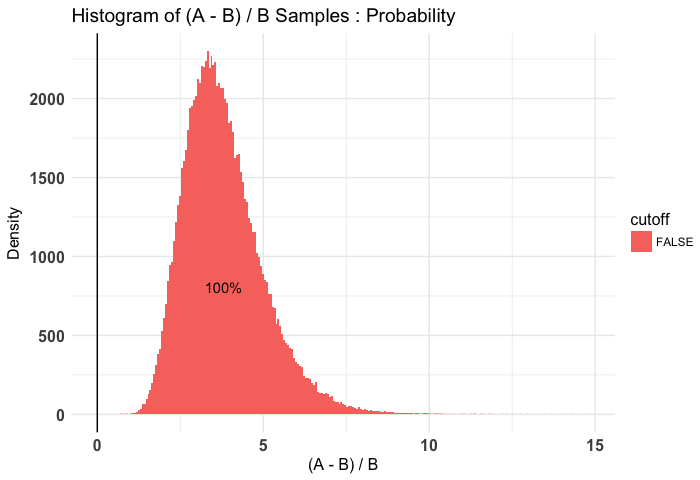
As we can see, it's somewhat clear that the diffuse is worse than the weak and very clear that the diffuse is worse than the stronger priors. Note that in our case I use a diffuse prior of Beta(1, 1) since I have no idea what's normal going into this simulation.
Finally we can check the output of summary to see if the Posterior Expected Loss is within our constraints.
summary(t1)## Quantiles of posteriors for A and B:
##
## $Probability
## $Probability$A_probs
## 0% 25% 50% 75% 100%
## 0.06019053 0.08936888 0.09552425 0.10188340 0.14012802
##
## $Probability$B_probs
## 0% 25% 50% 75% 100%
## 0.04926047 0.07582110 0.08158084 0.08758630 0.12639536
##
##
## --------------------------------------------
##
## P(A > B) by (0)%:
##
## $Probability
## [1] 0.86214
##
## --------------------------------------------
##
## Credible Interval on (A - B) / B for interval length(s) (0.9) :
##
## $Probability
## 5% 95%
## -0.07634565 0.48644269
##
## --------------------------------------------
##
## Posterior Expected Loss for choosing B over A:
##
## $Probability
## [1] 0.01270441summary(t2)## Quantiles of posteriors for A and B:
##
## $Probability
## $Probability$A_probs
## 0% 25% 50% 75% 100%
## 0.06244681 0.08940537 0.09554403 0.10195937 0.13931010
##
## $Probability$B_probs
## 0% 25% 50% 75% 100%
## 0.007008903 0.017726756 0.020601621 0.023791156 0.050439822
##
##
## --------------------------------------------
##
## P(A > B) by (0)%:
##
## $Probability
## [1] 1
##
## --------------------------------------------
##
## Credible Interval on (A - B) / B for interval length(s) (0.9) :
##
## $Probability
## 5% 95%
## 2.173703 5.994963
##
## --------------------------------------------
##
## Posterior Expected Loss for choosing B over A:
##
## $Probability
## [1] NaNIf the Posterior Expected Loss is lower than our threshold for caring on abs(A - B) then we can call this test and accept the current results. The PEL is small in both cases, and possibly 0/NaN for t2 so it's quite clear that priors, even weak ones, have a significant positive effect on Type 1 Errors. Remember that we see this effect partially because our priors were of a similar shape to the data. If the priors and the data disagree, the effects might not be so clear cut and you will need more data to have a stable posterior.
Check out bayesAB 0.7.0 to supercharge your AB tests and reach out to me if you have any questions!


