On the German Tank / Taxicab Problem

As a Statistician it naturally follows that getting the chance to use Statistics at work is surprisingly rare. That means that when I can actually use probability distributions and random variables to solve a real world problem I get very excited.

Recently, I had an opportunity to apply the 'Taxicab Problem' to something that came up at work. Given that I work for a ridesharing platform and I was quite literally counting "taxis" (or at least cars meant to drive others around), this was doubly exquisite.

For the uninitiated, the Taxicab / German Tank problem is as follows:

Viewing a city from the train, you see a taxi numbered x. Assuming taxicabs are consecutively numbered, how many taxicabs are in the city?

This was also applied to counting German tanks in World War II to know when/if to attack. Statstical methods ended up being accurate within a few tanks (on a scale of 200-300) while "intelligence" (unintelligence) operations overestimated numbers about 6-7x. Read the full details on Wikipedia here (and donate while you're over there).

Somebody suggested using \(2 * \bar{x}\) where \(\bar{x}\) is the mean of the current observations. This made the hair on the back of my neck stand up but outside of my quantitative spidey senses I couldn't analytically prove why this was a bad solution. On one hand, it makes some sense intuitively. If the distribution of the numbers you see is random, you can be somewhat sure that the mean of your subset is approximately the mean of the true distribution. Then you simply multiply by 2 to get the max since the distribution is uniform. However, this doesn't take into account that \(2 * \bar{x}\) might be lower than \(m\) where \(m\) is the max number you've seen so far. An easy fix to this method is to simply use \(max(m, 2 * \bar{x})\). Regarding analytic proofs (and my lack thereof) as to the asymptopic bounds here, I imagine you leverage some properties of normality (means are normally distributed with sufficient N).

To be most correct, we can use the MVUE (Minimum Variance Unbiased Estimator). I won't bore you with the derivation (and it's also on the Wiki), but it works out to be \(m + \frac{m}{N} - 1\) with \(m\) is again the max number you've seen and \(N\) is the total number you've seen. Let's compare all 3 methods below:

library(reshape2)
library(ggplot2)

trueMax <- 5000
n <- 500
draws <- 100

infer <- function(f) {
  replicate(n, {
    x <- sample(trueMax, draws, replace = F)
    f(x)
  }, simplify = "data.frame")
}

meanMethod <- infer(function(x) 2 * cumsum(x) / seq_along(x))
tankMethod <- infer(function(x) cummax(x) + (cummax(x) / seq_along(x)) - 1)
betterMeanMethod <- infer(function(x) {
  out <- 2 * cumsum(x) / seq_along(x)
  ifelse(out > cummax(x), out, cummax(x))
})

meanMethod <- melt(meanMethod)
tankMethod <- melt(tankMethod)
betterMeanMethod <- melt(betterMeanMethod)

meanMethod$method <- '2 * mean'
tankMethod$method <- 'm + m/N - 1'
betterMeanMethod$method <- 'max(m, 2 * mean)'

df <- rbind(meanMethod, tankMethod, betterMeanMethod)

Let's plot it:

qplot(Var1, value, group = interaction(Var2, method), color = method, data = df, geom = "line", alpha = I(.05)) +
  geom_hline(yintercept = 5000, size = 2, linetype = 2) +
  guides(colour = guide_legend(override.aes = list(alpha = 1))) +
  ylab("Best Guess") +
  xlab("How many have we seen so far?") +
  xlim(1, 100)

Zoom in a bit:

last_plot() + xlim(1, 25)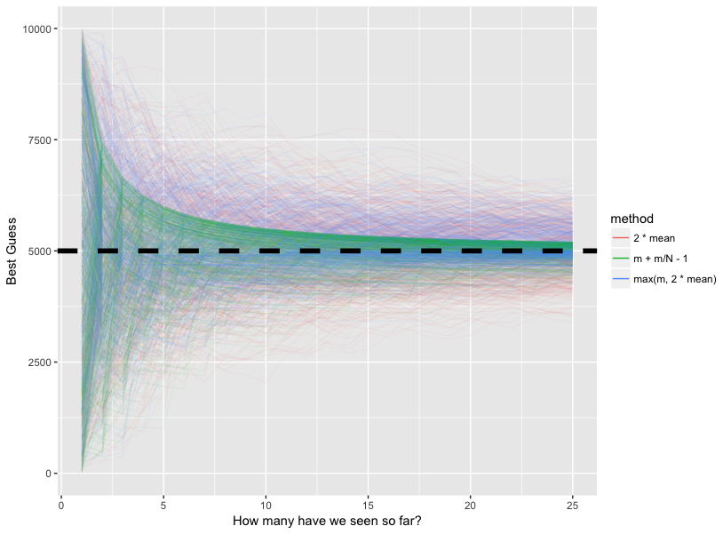

And this one is just prettttyyyy:

last_plot() + xlim(1, 5)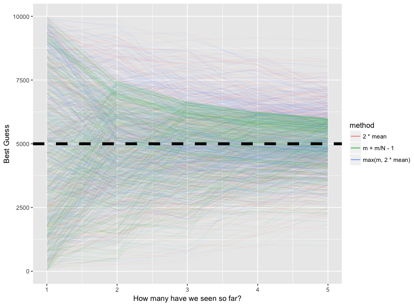

As we can see, the green line converges to the true max of 5000 very quickly, and has far less variance than the two other methods. The modified method I proposed is just an asymmetric version of \(2 * \bar{x}\), which approaches the true max but seems to level out in local minima/maxima at certain points. Ultimately, you can't deny that the MVUE method is best.

Another approach we can take is a Bayesian one. Since I'd never pass up an opportunity to self promote, let's use bayesAB (github repo here). This is actually an extra cool example since we show that bayesAB can be used to make inferences about a single posterior even the primary usecase of the package is for comparing sets of 2.

For brevity's sake, we fit a Bayesian model using the Pareto distribution as the conjugate prior (if this is all a foreign language to you, definitely check out my other blog posts on bayesAB 1 2). We can use very small values for xm and alpha as diffuse priors so the model we build for the Uniform distribution is solely based on the data.

x <- sample(trueMax, draws, replace = F)

mod <- bayesTest(x, x, priors = c("xm" = .005, "alpha" = .005), distribution = "uniform")

plot(mod, priors = FALSE, samples = FALSE)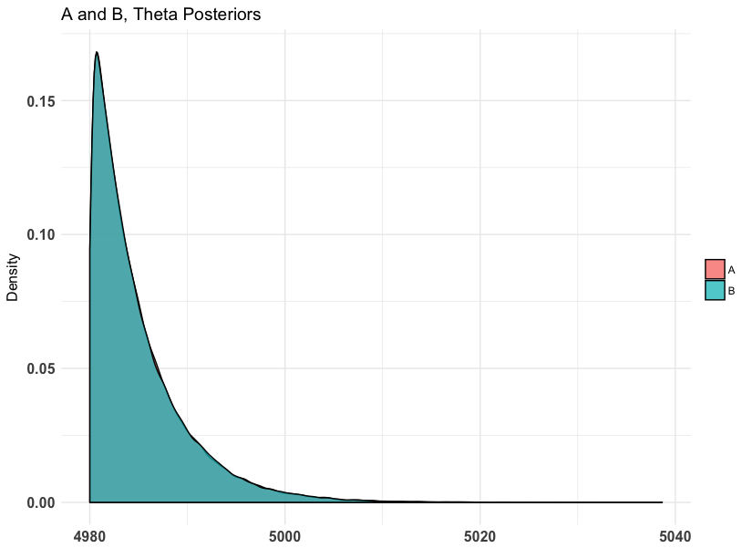

As we can see, the posterior is fairly thin between 4980 and 5000. Taking the mean or median of this is a solid estimate for the maximum. Let's see what the median says using the summary generic.

summary(mod)

Quantiles of posteriors for A and B:

$Theta
$Theta$A_thetas
      0%      25%      50%      75%     100% 
4980.000 4981.431 4983.458 4986.891 5038.651 

$Theta$B_thetas
      0%      25%      50%      75%     100% 
4980.000 4981.445 4983.448 4986.914 5036.582 


--------------------------------------------

P(A > B) by (0)%: 

$Theta
[1] 0.49782

--------------------------------------------

Credible Interval on (A - B) / B for interval length(s) (0.9) : 

$Theta
          5%          95% 
-0.002282182  0.002298932 

--------------------------------------------

Posterior Expected Loss for choosing B over A:

$Theta
[1] 2504.588

For our purposes, we can ignore everything besides the quantiles of the posteriors. Using this, we arrive at an estimate of 4983 as our max. Using \(2 * \bar{x}\) for this same sample results in 5034 which is overshooting by quite a bit.

Frank Portman