Update 2017-09-26: Please don't e-mail me asking to share the final model with you.
For one of my computational finance classes, I attempted to implement a Machine Learning algorithm in order to predict stock prices, namely S&P 500 Adjusted Close prices. In order to do this, I turned to Artificial Neural Networks (ANN) for a plethora of reasons. ANNs have been known to work well for computationally intensive problems where a user may not have a clear hypothesis of how the inputs should interact. As such, ANNs excel at picking up hidden patterns within the data so well that they often overfit!
Keeping this in mind, I experimented with a technique known as a 'sliding window'. Rather than train the model with years of S&P 500 data, I created an ANN that would train over the past 30 days (t-30, ..., t) to predict the close price at t+1. A 30 day sliding window seemed to make a good fit. It wasn't so wide as to not capture the current market atmosphere, but also it wasn't narrow enough to be hypersensitive to recent erratic movements.
Then, I had to decide on the input variables I was going to use. Many stock market models are pure time-series autoregressive functions, but the benefit of ANNs is that we can use them as a more traditional Machine Learning technique, we several inputs (and not only previous prices). This is helpful, because there exist an extremely large number of technical indicators which should uncover some significance in the market. I defined several of my own inputs that I thought would be significant predictors such as:
- 28 Day Moving Average
- 14 Day Moving Average
- 7 Day Moving Average
- Previous Day Close Price
In addition, I did some research and introduced several other technical indicators. Since there were so many, I fit a Random Forest model in order to reduce the dimensionality of the problem. After taking only the most important variables, I was left with:
- Volatility
- SAR
- MACD Oscillator
- ATR
Finally, in order to obtain a stable model, I had to scale the inputs so that all variables lied in the range of . This is done to avoid oversaturating the individual neurons in the ANN with outliers. There are several ways to do this, and I just created a simple function called 'myScale' in order to get the job done.
myScale <- function(x) {
  (x - min(x)) / (max(x) - min(x))
}
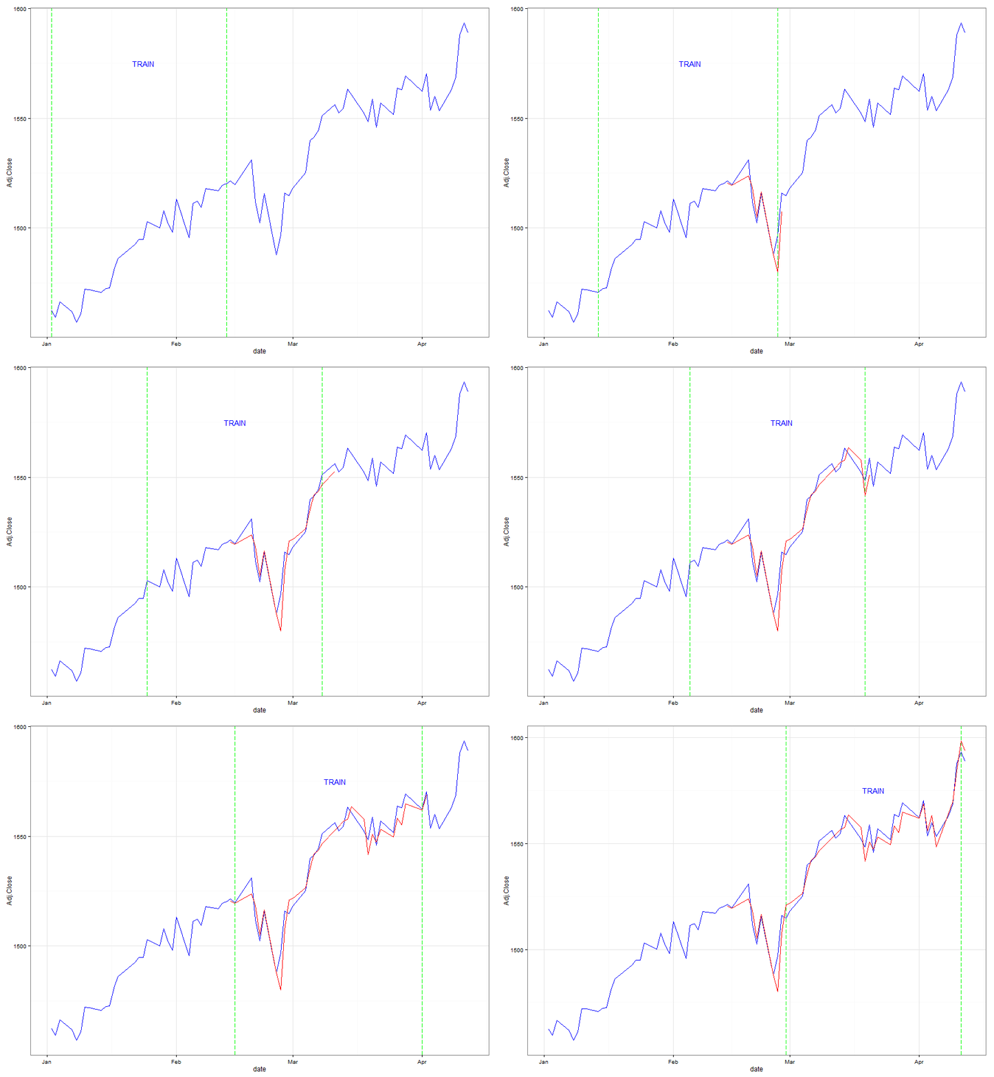
I won't be sharing the final model, but I did create a simulation of my methodology for the 2013 trading year.
trainPlot <- function(x) {

  g <- ggplot() + geom_path(aes(x = date, y = Adj.Close), colour = I("blue"),
                            data = sp.2013)

  g <- g + geom_vline(xintercept = as.numeric(sp.2013$date[x]), colour="green",
                      linetype = "longdash")

  g <- g + geom_vline(xintercept = as.numeric(sp.2013$date[x + 29]),
                      colour="green", linetype = "longdash")

  g <- g + annotate("text", x = sp.2013$date[x + 15], y = 1575,
                    label = "TRAIN", col = "blue")

  g <- g + geom_path(aes(x = date, y = Adj.Close), data = pred[31:(x + 30), ],
                     colour = I("red"))

  g <- g + theme_bw()

}

plotit <- function(x) print(trainPlot(x))

library(animation)
ani.options(ani.width = 900, ani.height = 650)

saveGIF(for (i in 1:40) plotit(i), convert = "gm convert",
        cmd.fun = shell, clean = T, outdir = getwd())
The animation demonstrates the mechanics of a Sliding Window model. We see that the 'Training' Window keeps moving up, regardless of whether the prediction was accurate or not. The RMSE of the model for the 2013 dates is 1.2115 which is extremely small considering the prices of the S&P 500 are over 1000. We know from the RMSE, and from the animation that the fit tends to be good. When the predicted values are slightly off, we can still see that the ANN usually correctly predicts the direction of the S&P 500 for that day. Perhaps in the future I will revisit this problem as a classification instead due to the results we're seeing.
The beauty of my result is that although this is a naive implementation of a sophisticated model, we can see that the results are really good. I can spend many weeks tuning the model and playing around with the inputs to get a better fit.


